Data Preparation#

author: Hamid Ali Syed
email: hamidsyed37[at]gmail[dot]com

import warnings
warnings.filterwarnings("ignore")
import requests
from bs4 import BeautifulSoup
import pandas as pd
import numpy as np

Data collection#

Let’s do some Web Scrapping#

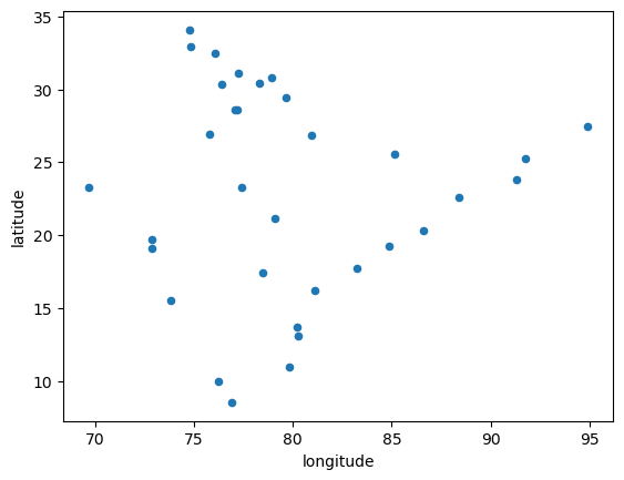
Let’s do some Web Scrapping. We can scrap the radar site information from the website of the Indian Meteorological Department (IMD) and extract location information from the HTML using BeautifulSoup. Then, we can clean and transform the extracted data into a Pandas DataFrame, with longitude and latitude coordinates for each location. Finally, we can plot the DataFrame as a scatter plot using longitude and latitude as x and y axes, respectively.

url = "https://mausam.imd.gov.in/imd_latest/contents/index_radar.php"
response = requests.get(url)
soup = BeautifulSoup(response.text, "html.parser")

# extract the relevant part of the HTML
images_html = soup.find_all("script")[-2].text.split("images: [")[0].split("],\n")[0]

# split the HTML into individual locations and extract the relevant information
locations = []
for image in soup.find_all("script")[-2].text.split("images: [")[0].split("],\n")[0].split("{")[1:]:
    location_dict = {}
    for line in image.split("\n"):
        if "title" in line:
            location_dict["title"] = line.split(": ")[-1].strip(',')
        elif "latitude" in line:
            location_dict["latitude"] = line.split(": ")[-1].strip(',')
        elif "longitude" in line:
            location_dict["longitude"] = line.split(": ")[-1].strip(',')
    locations.append(location_dict)

# create a DataFrame from the list of dictionaries
df = pd.DataFrame(locations)
df = df.dropna()
df['title'] = df['title'].str.strip(", ").str.strip('"')
df['longitude'] = df['longitude'].str.strip(", ").str.strip('longitude":')
df['latitude'] = df['latitude'].astype(float)
df['longitude'] = df['longitude'].astype(float)
df['title'].replace("Goa", "Panaji", inplace=True)
df.plot(kind='scatter', x='longitude', y='latitude')
df

	title	latitude	longitude
2	Bhopal	23.259900	77.412600
3	Agartala	23.831500	91.286800
4	Delhi	28.563200	77.191200
5	Bhuj	23.242000	69.666900
6	Chennai	13.082700	80.270700
7	Panaji	15.490900	73.827800
8	Gopalpur	19.264700	84.862000
9	Hyderabad	17.385000	78.486700
10	Jaipur	26.912400	75.787300
11	Kolkata	22.572600	88.363900
12	Kochi	9.931200	76.267300
13	Karaikal	10.925400	79.838000
14	Lucknow	26.846700	80.946200
15	Machilipatnam	16.190500	81.136200
16	Mumbai	19.076000	72.877700
17	Nagpur	21.145800	79.088200
18	Sohra	25.270200	91.732300
19	Patiala	30.339800	76.386900
20	Patna	25.594100	85.137600
21	Srinagar	34.083656	74.797371
22	Jammu	32.926600	74.857000
23	Thiruvananthapuram	8.524100	76.936600
24	Visakhapatnam	17.686800	83.218500
25	Mohanbari	27.472800	94.912000
26	Paradip	20.316600	86.611400
27	Sriharikota	13.725900	80.226600
28	Jot	32.486800	76.059300
29	Murari	30.789800	78.917850
30	Palam	28.590100	77.088800
31	Mukteshwar	29.460400	79.655800
32	Veravali	19.734300	72.876300
33	Kufri	31.097800	77.267800
34	Surkandaji	30.411400	78.288500

We have procured the name, lat, & lon info of all the radar sites and is saved in df. Now, let’s search for their frequency bands. I have found a webpage on the IMD website that contains this information for most of the radars. Let’s make a request to a URL and create a BeautifulSoup object to parse the HTML content. It will find a table on the page, then we can extract the headers and rows of the table, and create a Pandas DataFrame df2 from the table data.

Drop the "S No" column, clean up the "Type of DWR" and "DWR Station" columns by removing certain text, and replace some values in the "DWR Station" column.

# make a request to the URL
url = "https://mausam.imd.gov.in/imd_latest/contents/imd-dwr-network.php"
response = requests.get(url)

# create a BeautifulSoup object
soup = BeautifulSoup(response.content, "html.parser")

# find the table on the page
table = soup.find("table")

# extract the table headers
headers = [header.text.strip() for header in table.find_all("th")]

# extract the table rows
rows = []
for row in table.find_all("tr")[1:]:
    cells = [cell.text.strip() for cell in row.find_all("td")]
    rows.append(cells)

# create a DataFrame from the table data
df2 = pd.DataFrame(rows, columns=headers)
df2.drop("S No", axis=1, inplace=True)
df2['Type of DWR'] = df2['Type of DWR'].str.replace(' - Band', '')
df2['DWR Station'].replace('Delhi (Palam)', 'Palam', inplace=True)
df2['DWR Station'] = df2['DWR Station'].str.replace('\(ISRO\)', '').str.replace('\(Mausam Bhawan\)', 
                                                                                '').str.strip()
df2

	DWR Station	State	Type of DWR
0	Agartala	Tripura	S
1	Bhopal	Madhya Pradesh	S
2	Bhuj	Gujarat	S
3	Chennai	Tamil Nadu	S
4	Cherrapunjee	Meghalaya	S
5	Palam	Delhi	S
6	Panaji	Goa	S
7	Gopalpur	Odisha	S
8	Hyderabad	Telangana	S
9	Jaipur	Rajasthan	C
10	Kolkata	West Bengal	S
11	Kochi	Kerala	S
12	Karaikal	Tamil Nadu	S
13	Lucknow	Uttar Pradesh	S
14	Machilipatnam	Andhra Pradesh	S
15	Mohanbari	Assam	S
16	Mumbai	Maharashtra	S
17	Nagpur	Maharashtra	S
18	New Delhi	Delhi	C
19	Paradip	Odisha	S
20	Patiala	Punjab	S
21	Patna	Bihar	S
22	Srinagar	Jammu and Kashmir	X
23	Thiruvananthapuram	Kerala	C
24	Visakhapatnam	Andhra Pradesh	S

Let’s merge two previously created Pandas DataFrames, df and df2, using the “title” and “DWR Station” columns as keys, respectively. It will drop the “DWR Station” column, rename the “Type of DWR” column as “Band”, and replace some values in the “title” column. The code will count the number of NaN values in the “Band” column, print this count, and return the resulting merged DataFrame.

merged_df = df.merge(df2, left_on='title', right_on='DWR Station', how='left')
merged_df = merged_df.drop(columns=['DWR Station'])
merged_df = merged_df.rename(columns={'Type of DWR': 'Band'})
merged_df['title'].replace("Goa", "Panaji", inplace=True)
num_nans = merged_df['Band'].isna().sum()
print(num_nans)
merged_df

	title	latitude	longitude	State	Band
0	Bhopal	23.259900	77.412600	Madhya Pradesh	S
1	Agartala	23.831500	91.286800	Tripura	S
2	Delhi	28.563200	77.191200	NaN	NaN
3	Bhuj	23.242000	69.666900	Gujarat	S
4	Chennai	13.082700	80.270700	Tamil Nadu	S
5	Panaji	15.490900	73.827800	Goa	S
6	Gopalpur	19.264700	84.862000	Odisha	S
7	Hyderabad	17.385000	78.486700	Telangana	S
8	Jaipur	26.912400	75.787300	Rajasthan	C
9	Kolkata	22.572600	88.363900	West Bengal	S
10	Kochi	9.931200	76.267300	Kerala	S
11	Karaikal	10.925400	79.838000	Tamil Nadu	S
12	Lucknow	26.846700	80.946200	Uttar Pradesh	S
13	Machilipatnam	16.190500	81.136200	Andhra Pradesh	S
14	Mumbai	19.076000	72.877700	Maharashtra	S
15	Nagpur	21.145800	79.088200	Maharashtra	S
16	Sohra	25.270200	91.732300	NaN	NaN
17	Patiala	30.339800	76.386900	Punjab	S
18	Patna	25.594100	85.137600	Bihar	S
19	Srinagar	34.083656	74.797371	Jammu and Kashmir	X
20	Jammu	32.926600	74.857000	NaN	NaN
21	Thiruvananthapuram	8.524100	76.936600	Kerala	C
22	Visakhapatnam	17.686800	83.218500	Andhra Pradesh	S
23	Mohanbari	27.472800	94.912000	Assam	S
24	Paradip	20.316600	86.611400	Odisha	S
25	Sriharikota	13.725900	80.226600	NaN	NaN
26	Jot	32.486800	76.059300	NaN	NaN
27	Murari	30.789800	78.917850	NaN	NaN
28	Palam	28.590100	77.088800	Delhi	S
29	Mukteshwar	29.460400	79.655800	NaN	NaN
30	Veravali	19.734300	72.876300	NaN	NaN
31	Kufri	31.097800	77.267800	NaN	NaN
32	Surkandaji	30.411400	78.288500	NaN	NaN

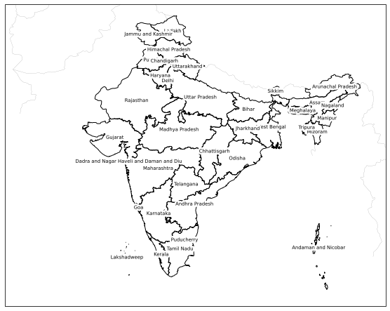
Since there are NaN values in the “State” column, we can find the state names using lat and lon info. We can use the Cartopy library to create a map of India with state boundaries and labels. Then we will create a pandas DataFrame gdf containing the latitude and longitude coordinates of each state and union territory, and try to map the names of these places in the merged_df

import cartopy.io.shapereader as shpreader
import geopandas as gpd
# Load the Natural Earth dataset
states_shp = shpreader.natural_earth(resolution='10m',
                                     category='cultural',
                                     name='admin_1_states_provinces')

import cartopy.crs as ccrs
import cartopy.io.shapereader as shpreader
import cartopy.feature as feat

import matplotlib.pyplot as plt
import matplotlib.patheffects as PathEffects

# get the data
fn = shpreader.natural_earth(
    resolution='10m', category='cultural', 
    name='admin_1_states_provinces',
)
reader = shpreader.Reader(fn)
states = [x for x in reader.records() if x.attributes["admin"] == "India"]
states_geom = feat.ShapelyFeature([x.geometry for x in states], ccrs.PlateCarree())

data_proj = ccrs.PlateCarree()

# create the plot
fig, ax = plt.subplots(
    figsize=(10,10), dpi=70, facecolor="w",
    subplot_kw=dict(projection=data_proj),
)

ax.add_feature(feat.BORDERS, color="k", lw=0.1)
# ax.add_feature(feat.COASTLINE, color="k", lw=0.2)
ax.set_extent([60, 100, 5, 35], crs=ccrs.Geodetic())

ax.add_feature(states_geom, facecolor="none", edgecolor="k")

# # add the names
for state in states:
    lon = state.geometry.centroid.x
    lat = state.geometry.centroid.y
    name = state.attributes["name"] 
    
    ax.text(
        lon, lat, name, size=7, transform=data_proj, ha="center", va="center",
        path_effects=[PathEffects.withStroke(linewidth=5, foreground="w")]
    )

locs = {}
for state in states:
    lon = state.geometry.centroid.x
    lat = state.geometry.centroid.y
    name = state.attributes["name"]
    locs[name] = {"lat": lat, "lon": lon}
gdf = pd.DataFrame(locs, ).T
gdf.reset_index(inplace=True)
gdf = gdf.rename({'index':'state'}, axis=1)
gdf.index = np.arange(1, len(gdf) + 1)

gdf

	state	lat	lon
1	Ladakh	33.885957	77.634965
2	Arunachal Pradesh	28.035900	94.660514
3	Sikkim	27.572023	88.448173
4	West Bengal	23.805249	87.972564
5	Assam	26.356938	92.831287
6	Uttarakhand	30.163721	79.196121
7	Nagaland	26.059820	94.448403
8	Manipur	24.730388	93.861591
9	Mizoram	23.292031	92.819139
10	Tripura	23.754753	91.728537
11	Meghalaya	25.536122	91.287036
12	Punjab	30.848293	75.404354
13	Rajasthan	26.592714	73.834251
14	Gujarat	22.712829	71.558165
15	Himachal Pradesh	31.936310	77.220849
16	Jammu and Kashmir	33.557813	75.079701
17	Bihar	25.662102	85.604230
18	Uttar Pradesh	26.934734	80.541922
19	Andhra Pradesh	15.721672	79.924211
20	Odisha	20.517113	84.414536
21	Dadra and Nagar Haveli and Daman and Diu	20.199380	72.992494
22	Maharashtra	19.460457	76.111348
23	Goa	15.352195	74.045828
24	Karnataka	14.719826	76.155168
25	Kerala	10.423815	76.424882
26	Puducherry	11.960162	78.885684
27	Tamil Nadu	11.014705	78.402304
28	Lakshadweep	10.120942	72.827601
29	Andaman and Nicobar	11.133776	92.975529
30	Jharkhand	23.642010	85.533387
31	Delhi	28.660865	77.107946
32	Chandigarh	30.743535	76.768380
33	Madhya Pradesh	23.539092	78.292780
34	Chhattisgarh	21.255901	82.033368
35	Haryana	29.208370	76.336467
36	Telangana	17.796650	79.050764

# merged_df.sort_values(by=['latitude', 'longitude'], ascending=False)

merged_df = df.merge(df2, left_on='title', right_on='DWR Station', how='left')
merged_df = merged_df.drop(columns=['DWR Station'])
merged_df = merged_df.rename(columns={'Type of DWR': 'Band'})
merged_df

	title	latitude	longitude	State	Band
0	Bhopal	23.259900	77.412600	Madhya Pradesh	S
1	Agartala	23.831500	91.286800	Tripura	S
2	Delhi	28.563200	77.191200	NaN	NaN
3	Bhuj	23.242000	69.666900	Gujarat	S
4	Chennai	13.082700	80.270700	Tamil Nadu	S
5	Panaji	15.490900	73.827800	Goa	S
6	Gopalpur	19.264700	84.862000	Odisha	S
7	Hyderabad	17.385000	78.486700	Telangana	S
8	Jaipur	26.912400	75.787300	Rajasthan	C
9	Kolkata	22.572600	88.363900	West Bengal	S
10	Kochi	9.931200	76.267300	Kerala	S
11	Karaikal	10.925400	79.838000	Tamil Nadu	S
12	Lucknow	26.846700	80.946200	Uttar Pradesh	S
13	Machilipatnam	16.190500	81.136200	Andhra Pradesh	S
14	Mumbai	19.076000	72.877700	Maharashtra	S
15	Nagpur	21.145800	79.088200	Maharashtra	S
16	Sohra	25.270200	91.732300	NaN	NaN
17	Patiala	30.339800	76.386900	Punjab	S
18	Patna	25.594100	85.137600	Bihar	S
19	Srinagar	34.083656	74.797371	Jammu and Kashmir	X
20	Jammu	32.926600	74.857000	NaN	NaN
21	Thiruvananthapuram	8.524100	76.936600	Kerala	C
22	Visakhapatnam	17.686800	83.218500	Andhra Pradesh	S
23	Mohanbari	27.472800	94.912000	Assam	S
24	Paradip	20.316600	86.611400	Odisha	S
25	Sriharikota	13.725900	80.226600	NaN	NaN
26	Jot	32.486800	76.059300	NaN	NaN
27	Murari	30.789800	78.917850	NaN	NaN
28	Palam	28.590100	77.088800	Delhi	S
29	Mukteshwar	29.460400	79.655800	NaN	NaN
30	Veravali	19.734300	72.876300	NaN	NaN
31	Kufri	31.097800	77.267800	NaN	NaN
32	Surkandaji	30.411400	78.288500	NaN	NaN

from math import radians, sin, cos, sqrt, asin

# Function to calculate the haversine distance between two coordinates in km
def haversine(lat1, lon1, lat2, lon2):
    R = 6371  # radius of Earth in km
    dLat = radians(lat2 - lat1)
    dLon = radians(lon2 - lon1)
    lat1 = radians(lat1)
    lat2 = radians(lat2)
    a = sin(dLat/2)**2 + cos(lat1)*cos(lat2)*sin(dLon/2)**2
    c = 2*asin(sqrt(a))
    return R*c

# Loop through each row in merged_df
for i, row in merged_df.iterrows():
    if pd.isna(row["State"]):
        min_dist = float('inf')
        closest_state = ""
        # Loop through each row in gdf to find the closest one
        for j, gdf_row in gdf.iterrows():
            dist = haversine(row["latitude"], row["longitude"], gdf_row["lat"], gdf_row["lon"])
            if dist < min_dist:
                min_dist = dist
                closest_state = gdf_row["state"]
        merged_df.at[i, "State"] = closest_state

merged_df.sort_values(by = "latitude", ascending=False)

	title	latitude	longitude	State	Band
19	Srinagar	34.083656	74.797371	Jammu and Kashmir	X
20	Jammu	32.926600	74.857000	Jammu and Kashmir	NaN
26	Jot	32.486800	76.059300	Himachal Pradesh	NaN
31	Kufri	31.097800	77.267800	Chandigarh	NaN
27	Murari	30.789800	78.917850	Uttarakhand	NaN
32	Surkandaji	30.411400	78.288500	Uttarakhand	NaN
17	Patiala	30.339800	76.386900	Punjab	S
29	Mukteshwar	29.460400	79.655800	Uttarakhand	NaN
28	Palam	28.590100	77.088800	Delhi	S
2	Delhi	28.563200	77.191200	Delhi	NaN
23	Mohanbari	27.472800	94.912000	Assam	S
8	Jaipur	26.912400	75.787300	Rajasthan	C
12	Lucknow	26.846700	80.946200	Uttar Pradesh	S
18	Patna	25.594100	85.137600	Bihar	S
16	Sohra	25.270200	91.732300	Meghalaya	NaN
1	Agartala	23.831500	91.286800	Tripura	S
0	Bhopal	23.259900	77.412600	Madhya Pradesh	S
3	Bhuj	23.242000	69.666900	Gujarat	S
9	Kolkata	22.572600	88.363900	West Bengal	S
15	Nagpur	21.145800	79.088200	Maharashtra	S
24	Paradip	20.316600	86.611400	Odisha	S
30	Veravali	19.734300	72.876300	Dadra and Nagar Haveli and Daman and Diu	NaN
6	Gopalpur	19.264700	84.862000	Odisha	S
14	Mumbai	19.076000	72.877700	Maharashtra	S
22	Visakhapatnam	17.686800	83.218500	Andhra Pradesh	S
7	Hyderabad	17.385000	78.486700	Telangana	S
13	Machilipatnam	16.190500	81.136200	Andhra Pradesh	S
5	Panaji	15.490900	73.827800	Goa	S
25	Sriharikota	13.725900	80.226600	Andhra Pradesh	NaN
4	Chennai	13.082700	80.270700	Tamil Nadu	S
11	Karaikal	10.925400	79.838000	Tamil Nadu	S
10	Kochi	9.931200	76.267300	Kerala	S
21	Thiruvananthapuram	8.524100	76.936600	Kerala	C

# Merge merged_df and df2 on the "State" column
merged_df_with_band = pd.merge(merged_df, df2[['State', 'Type of DWR']], on='State', how='left')

# Replace NaN values in the "Band" column with corresponding values from the "Type of DWR" column
merged_df_with_band['Band'].fillna(merged_df_with_band['Type of DWR'], inplace=True)

# Drop the "Type of DWR" column
merged_df_with_band.drop('Type of DWR', axis=1, inplace=True)

merged_df_with_band.drop(2, inplace=True)

merged_df_with_band.drop_duplicates("latitude", inplace=True)
merged_df_with_band.drop_duplicates("longitude", inplace=True)
merged_df_with_band.sort_values(by="latitude", ascending=False, inplace=True)

merged_df_with_band.index = np.arange(1, len(merged_df_with_band)+1, 1)

f_df = merged_df_with_band.copy()

f_df.loc[f_df['title'] == 'Veravali', 'Band'] = 'C'

nan_mask = f_df['Band'].isna()
nan_df = f_df[nan_mask]
nan_df.loc[:, 'Band'] = nan_df['Band'].fillna('X')
f_df.update(nan_df)

f_df.rename(columns={'title': 'Site',
                     "latitude": "Latitude", 
                     "longitude":"Longitude"}, inplace=True)

f_df.attrs["Range"]={"C":250,
                    "X":100,
                    "S":250
                   }

f_df.to_csv("IMD_Radar_Sites_2022.csv")

IMD Radar Network

Data Preparation

Contents

Data Preparation#

Data collection#

Let’s do some Web Scrapping#